Sometimes linear regression doesn’t quite cut it – particularly when we believe that our observed relationships are non-linear.  For this reason, we should turn to other types of regression.  This page is a brief lesson on how to calculate a quadratic regression in Python.  As always, if you have any questions, please email me at MHoward@SouthAlabama.edu!

---

The typical type of regression is a linear regression, which identifies a linear relationship between predictor(s) and an outcome.  Sometimes our effects are non-linear, however.  In these cases, we need to apply different types of regression.

A common non-linear relationship is the quadratic relationship, which is a relationship that is described by a single curve.  In these instances, the relationship between two variables may look like a U or an upside-down U.  Often, we call the latter of these relationships (the upside down U) a “too much of a good thing” effect.  That is, when one variable goes up, then the other goes up too; however, once you get to a certain point, the relationship goes back down.  For example, conscientiousness may relate to life satisfaction.  If you are hard working, then you are generally happier with your life.  However, once you get to a certain level of conscientiousness, your life satisfaction might go back down.  If you are too hard working, then you may be stressed and less happy with your life.

There is more that could be stated about quadratic regression, but we’ll keep it simple.  To calculate a quadratic regression, we can use Python.  If you don’t have a dataset, you can download the example dataset here.  Using this dataset, we are going to investigate the linear and quadratic relationship of Var2 predicting Var1.

We are going to be using the pingouin and pandas modules. If you don’t know how to install modules, you can look at my guide for installing Python modules here. Likewise, you need to open your .csv file with Python. If you don’t know how to do so, you can look at my guide for opening .csv files in Python. Lastly, the example dataset is a .xslx file. You can look at this guide on how to convert .xlsx files to .csv files by clicking here.

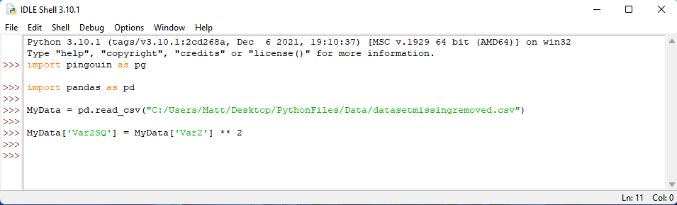
With that noted, your syntax should begin with the following:

To perform our analysis, we first need to create the new variable that will detect the non-linear effect. For a quadratic regression, this is our predictor squared (Var2^2). We will call it, Var2SQ, in this example. To create this variable, we need to first provide this new label by typing: MyData[‘Var2SQ’] = . Then, we need to tell Python that this new variable should be the square of Var2. To do so, we type: MyData[‘Var2’] ** 2. In Python, ** is used to take a variable to the power of the following number. So, ** 2 indicates that the variable should be squared. Once you have written this syntax, press enter.

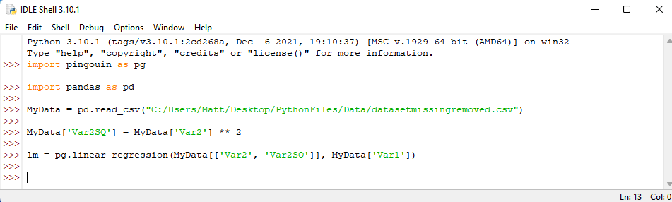
We should then conduct our regression analyses with Var 1 as our outcome and Var2 and Var2SQ as our predictors. If you do not know how to conduct a regression analysis in Python, please refer to my page on the topic. In short, however, we want to assign our regression results to lm by typing the following syntax: lm = pg.linear_regression(MyData[[‘Var2’, ‘Var2SQ’]], MyData[‘Var1’]) . We then press enter.

Afterwards, we tell Python to provide our regression results when rounded to two decimal places. We do this by typing the following: lm.round(2) . Press enter.

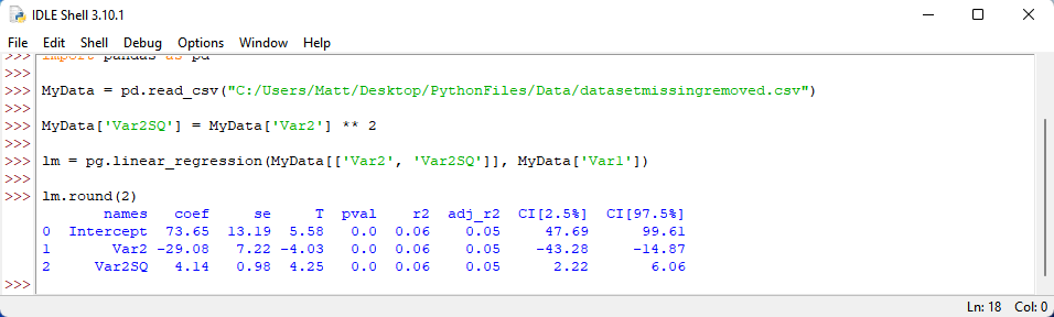
Did you get these results?  Or something similar?  From these results, we can see that the quadratic effect, Var2SQ, was indeed statistically significant.  So, we could say that a non-linear relationship exists between Var2 and Var1.  Pretty neat!

More information about interpreting regression output in Python can be obtained from my page on performing a regression in Python.  If you have any questions or comments about performing a regression in Python, please contact me at MHoward@SouthAlabama.edu.