In every class that I teach, even statistics, I assign a research paper. For the most part, students do a superb job reviewing relevant research articles and integrating several themes; however, when reporting statistical results, students (most of the time) only note p-values. This is likely for two reasons.

First, p-values are amongst the (deceivingly) easiest statistical concepts to understand. Students usually view p-values as an on-off switch. If the p-value is significant, then the switch is on and they should pay attention to the result. If the p-value is not significant, then the switch is off and they should not pay attention to the result. This logic is problematic and is often not true. Some significant results may not be important, and many non-significant results are very important – But when? Second, some statistics classes tend to cut corners. Instead of teaching about effect sizes, a focus is only given to p-values as they are perceived as more universal. Once again, this is problematic. Students should be able to interpret the statistical results themselves rather than just the corresponding p-value, as the results often provide more information than the p-value.

Given the reoccurring confusion and controversy over p-values, I review the meaning of p-values. After the review, any reader should have a general understanding of p-values. Then, I review the controversies of p-values which led APA to create their first ever taskforce to discuss the potential harms of p-values – even before they created a taskforce on several other important topics, such as “Don’t Ask, Don’t Tell” and “Mental Disability and the Death Penalty.” After this
discussion, a reader could consider themselves in-the-know about p-values.

Meaning

The meaning of a p-value is (seemingly) simple: A p-value is the probability that the observed data (or more extreme data) would have occurred if we assume that the null hypothesis is true. For instance, when performing a t-test which compares two groups of data, such as the test scores for two classrooms, the p-value indicates the likelihood that the observed differences between the two groups (or larger differences) would have occurred due to random chance if we assume that the null hypothesis is true. If the p-value is 0.05, for example, it indicates that there is a five percent likelihood that we would have observed our results (or more extreme results) assuming that the null hypothesis is true. So what does this mean for a research study?

When researchers study a topic, they create hypotheses. The proposed hypothesis is called the research or alternative hypothesis, and it proposes that an effect exists. In the classroom example, the research hypothesis may be that students in Classroom 1 perform better on tests compared to Classroom 2. When reporting studies, researchers directly state their research hypotheses. The research hypothesis is pitted against the null hypothesis, which proposes that the effect does not exist. In the classroom example, the research hypothesis may be that students in Classroom 1 perform equal on tests compared to Classroom 2. Often, the null hypothesis is not directly stated, but it is implied.

To support the research hypothesis, we must be able to say that an effect is significantly different from random chance. When an effect is different than random chance, something other than randomness is affecting the dynamic of interest, such as test scores within the classrooms. This is why researchers claim that “The null was rejected” when they find significant results– they are saying that the data probably did not occur to random chance, a notable effect is likely present, and the p-value was less than 0.05. This logic is the basis for Null Hypothesis Significance Testing (NHST), which is the development and testing of hypotheses based upon p-values.

In general, researchers only report if the p-value is below a certain level, often 0.05, for two reasons. First, researchers have generally agreed that any results with greater than a five percent chance to be due to randomness when assuming that the null hypothesis is true (p > .05), then the results are too unreliable and should not be considered different from random chance alone. Other p-values are generally not of interest, but authors will report if a p-value is smaller than .01, .001, or .0001. Second, p-values are always continuous numbers and cannot be completely written-out. Researchers could write their p-values as, “p = .045…” or “p ≈ .045,” but they choose to not. So, the standard convention is to write whether p-values are lower than a certain cutoff, with the conventional values being .05, .01, .001, and .0001.  AUTHOR NOTE: This is now changing in the social sciences – write out your p-values!

Right now, this explanation may seem simple, but let’s look into how p-values are calculated.

Three components are involved in the calculation of a p-value for most statistical tests: the magnitude, the variance, and the sample size. The magnitude refers to the size of the actual statistical result. In the classrooms example, the magnitude would be the difference between the average test scores of the two groups. For example, the average of Classroom 1 may be four whereas the average of Classroom 2 may be six, which results in a magnitude of two. In general, when the magnitude is large, the results are more likely to be statistically significant.

The variance refers to the size of data’s distributions. In the classrooms example, the variance would be the distribution of scores within the two classes. For example, although the averages were four and six, students’ scores may have (theoretically) ranged from four to six, 0 to 10, -100 to 100, or almost anything else which includes the values four and six. In general, when the variance is small, the results are more likely to be statistically significant.

Lastly, the sample size refers to the number of observations within the data. In the classrooms example, the sample size would be the number of students within each class. For example, the two classrooms may have 10 students, 100 students, or 1000 students. In general, when the sample size is large, the results are more likely to be statistically significant.

Still confused? That is okay. The pictures and explanation below might help.

In Chart 1, the x-axis is the test score, the y-axis is the number of students receiving that score, and the different colors represent the difference classes. The two classrooms have ten students each, and I randomly generated the data from the same distribution. That means that the data was taken from a distribution with the same mean (six) and variance (range of ten). The two groups should not be statistically different or significant, and any observed differences are due to complete random chance. When looking at the data, it appears similar. Nevertheless, we cannot be sure without statistical tests. When performing a t-test on the two groups (t = 0.903, df = 18, Std. Err. = 1.551), the results are not statistically significant (p > .05). We are unable to reject the null hypothesis, and any difference between the groups is believed to be due to random chance.

In Chart 2, the two classrooms have ten students each, and I randomly generated the data from different distributions. In Classroom 1, the data was randomly taken from a range between 1 and 7. In Classroom 2, the data was
random taken from a range between 3 and 9. While the distributions of the data have the same variance (range of six), they have different means (four and six). The two groups should be statistically different or significant. When looking at the data, however, the data appears fairly similar. When performing a t-test on the two groups (t = 1.681, df = 18, Std. Err. = 0.833), the results are not statistically significant (p > .05). We are unable to reject the null hypothesis, and any
difference between the groups is believed to be due to random chance.

But why? The means of the distributions that created the data were different – shouldn’t the results reflect a difference between the two groups? It is probably because of the small sample sizes. With only 20 students, total, it is difficult to determine whether the two groups are actually different.

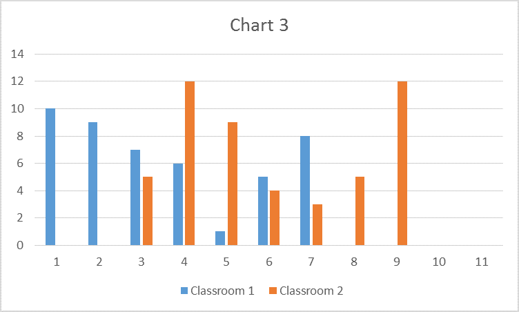Now, in Chart 3, the two classrooms have 50 students each. The data was generated from the same distributions as Chart 2. Once again, the two groups should be statistically different or significant. When looking at the data, this is clear. They appear, in fact, different. When performing a t-test on the two groups (t = 5.413, df = 98, Std. Err. = 0.432), the results are statistically significant (p < .001). We are able to reject the null hypothesis, and we believe that the difference between the two groups is likely due to an actual effect. The differences between Charts 2 and 3 largely arise from the sample sizes.

Let’s take one last example in Chart 4. In Chart 4, each group still had 50 students, and the data was generated from different distributions. Each distribution still had a difference of two (means of nine and eleven); however, the variances of each group were increased (range of 16). Whereas the two groups previously had a range of six, the two groups now have a range of 16. Given that the means of the two groups are different, they should be statistically different or significant. When looking at the data, it is unclear if this is true. When performing a t-test on the two groups (t = 1.380, df = 98, Std. Err. = 1.007), the results are not statistically significant (p > .05). We are unable to reject the null hypothesis, and any difference between the groups is believed to be due to random chance. This is because the large variances extensively overlap, making it unclear whether the two groups actually statistically differ.

Phew! That was a lot, but I hope it clears things up. At this point, what do you think of p-values? Do you think they are useful inferences into the significance of our data? Or are they misleading?

Also, if you are still confused about p-values, please email me at MHoward@SouthAlabama.edu. Hopefully I can change the explanation to clarify things. Also, I should make two quick notes about the explanation above.

First, my discussion was focused on p-values for t-tests. I believe that p-values in t-tests are the easiest to understand; however, p-values can correspond to an array of other statics, including correlations, ANOVAS, structural equation
modeling, and many others. When analyzing p-values for these statistics, the logic is largely the same. Second, the data for the examples above was sampled from a uniform distribution, not a normal distribution, once again to aid in
understanding. That is why variance was discussed in ranges rather than standard deviations. Once you become more familiar with p-values, you should look into the relationship of standard deviations and p-values, and you should replicate the results above with normal distributions.

With a basic understanding of p-values achieved, let’s look into the controversies surrounding p-values.