Regression is a powerful tool.  Fortunately, regressions can be calculated easily in Jamovi.  This page is a brief lesson on how to calculate a regression in Jamovi.  As always, if you have any questions, please email me at MHoward@SouthAlabama.edu!

---

The typical type of regression is a linear regression, which identifies a linear relationship between predictor(s) and an outcome.  In other words, a regression can tell you the relatedness of one or many predictors with a single outcome.  Regression also tests each of these relationships while controlling for the other predictors, and it can be used to answer the following questions and similar others:

• What is the relationship of job satisfaction and leader ability in predicting employee job satisfaction?
• What is the relationship of hours studied and test grades?
• What is the relationship between NBA player height, weight, wingspan and the number of points scored per game?

Of course, there is more nuance to regression, but we will keep it simple.  To answer these questions, we can use Jamovi to calculate a regression equation.  If you don’t have a dataset, you can download the example dataset here. In the dataset, we are investigating the relationships of job satisfaction and social desirability with job performance.

Also, this file is in .xls format, but Jamovi cannot open this format.  To learn how to change this .xls file to a .csv file, which Jamovi can open, please click here.  Also, the pictures below are a little small on the page. Click on the link above each picture to view a larger version of the picture in a new window.

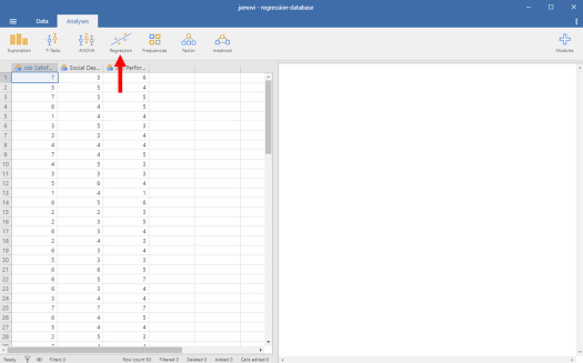
The data should look something like this:

Regression in Jamovi Picture 1

To start, click on the Regression button.

Regression in Jamovi Picture 2

Then click on Linear Regression.

Regression in Jamovi Picture 3

You should now see a window that looks like this:

Regression in Jamovi Picture 4

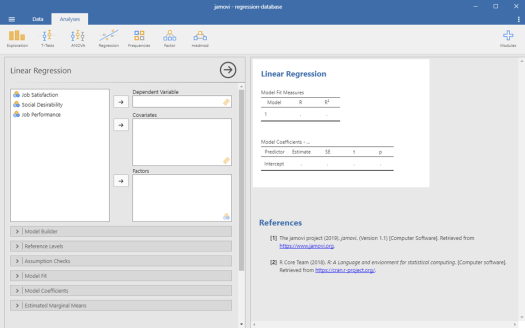
To start, let’s identify our outcome variable in Jamovi.  To do this, we select our outcome variable and designate it as the dependent variable.  In the current example, we want to select job performance and then click on the right-facing arrow next to the “Dependent Variable” box.

Regression in Jamovi Picture 5

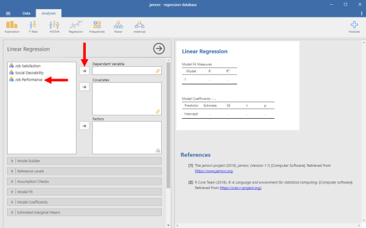
Now, let’s identify our predictor variables in Jamovi.  To do so, we want to select our predictor variables and designate them as covariates.  In the current example, we want to select job satisfaction and social desirability.  We then want to click on the right-facing arrow next to the “Covariates” box.

Regression in Jamovi Picture 6

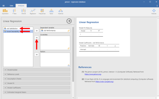
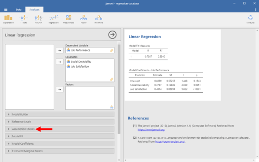
And we get some initial regression results!  Before interpreting them, however, there are some options that I want to click.

First, I want to see whether multicolinearity is an issue in my regression results.  To obtain relevant indicators of multicolinearity, click on the “Assumption Checks” tab.

Regression in Jamovi Picture 7

A new pop out window should appear, as seen below:

Regression in Jamovi Picture 8

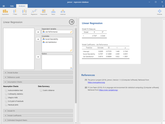
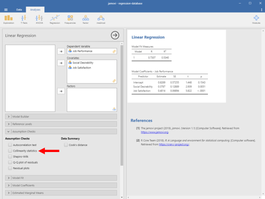
From here, click on the box next to “Collinearity statistics”.

Regression in Jamovi Picture 9

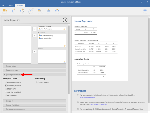
Now we need one final statistic – the standardized beta coefficients.  Go ahead and close that tab by clicking on the “Assumption Checks” bar again.

Regression in Jamovi Picture 10

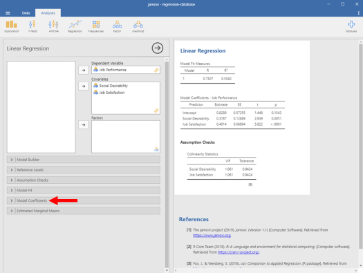
With that window closed, now we want to open the Model Coefficients window.  To do so, click on the “Model Coefficients” tab.

Regression in Jamovi Picture 11

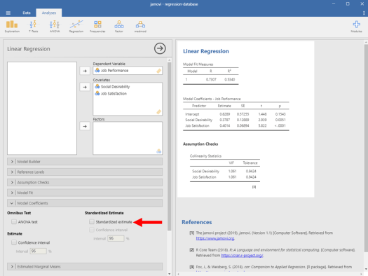
Finally, from this menu, click on the box next to “Standardized Estimate”.  This will provide our standardized beta coefficients.

Regression in Jamovi Picture 12

And there we go!  Now we have the statistics that we need.  Check the image below to ensure that your results are the same as mine.

Regression in Jamovi Picture 13

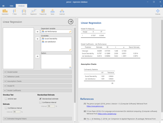
From these results,we should first look at our assumption checks, which is the very last table.  Our VIF value for both predcitors was 1.06.  There are a lot of different cutoffs for VIF.  Some authors say that VIF should be no higher than 3, 4, 5, or even 10.  Whichever cutoff that you choose, none of them are smaller than 1.06.  So, multicolinearity is not an issue with our data.

In the first table, we can also see that our R^2 is rather large at .53.  This means that our two predictors explain 53% of the variance in job performance.

Next, we can look at the p-value column on the second table to see the significance of our predictors.  We see that the p-value is less than .05 for both social desirability and job satisfaction.  That means that both social desirability and job satisfaction are statistically significant predictors of job performance.

Lastly, we can observe the nature of these relationships by looking at our standardized estimate column in the second table.  The standardized beta coefficient associated with social desirability was .30, whereas the coefficient associated with job satisfaction was .60.  This indicates that both predictors had strong and positive relations with job performance, and job satisfaction was a stronger predictor than social desirability.

Phew!  That was a lot!  From this page, you should be able to perform a regression analysis in Jamovi.  As always, if you have any questions or comments, please email me a MHoward@SouthAlabama.edu!