
Regression can provide numerical estimates of the relationships between multiple predictors and an outcome. It can also allow researchers to predict the value of an outcome given specific values of the predictors. This page provides a step-by-step guide on how to use regression for prediction in Excel. If you have any questions after reading, please email me at MHoward@SouthAlabama.edu.
Regression determines the liner relationship between predictor(s) and an outcome. If you need a refresher on regression, please check out my other guide on Regression in Excel. Once you obtain your regression results, specifically your unstandardized beta coefficients, you can use these results to estimate values of the outcome given specified values of the predictor(s). For instance, you could use regression to…
- Estimate the value of job performance given specific values of job satisfaction and conscientiousness.
- Estimate a company’s revenue given its market share and location.
- Estimate someone’s weight given their height.
The list of examples could go on and on. To estimate a value of the outcome given certain values of the predictor(s), however, we need to first conduct a regression analysis. If you don’t have a dataset, you can download the example dataset here. In the dataset, we are investigating the relationships of job satisfaction and social desirability with job performance. Go ahead and run your regression using all the predictors. In the example, it would be job satisfaction and social desirability predicting job performance. If you need help conducting this analysis for this example, please refer to my guide on Regression in Excel.
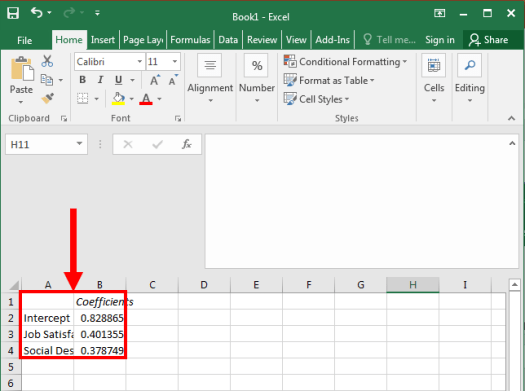
The results of your regression should look like the following:

We will want to predict the outcome by using the unstandardized beta coefficients, which are just labeled “coefficients” in the Excel output. We multiply these coefficients by the specified values of the predictors to predict our outcome. As you can see, the unstandardized regression equation from these results was: y = .829 + .401(JS) + .379(SD). So, we are going to use Excel to multiply .401*JS as well as .379*SD, before adding all of it together to obtain our predicted value. If you are confused by this, be sure to check out my YouTube video on “Inferences with Regression”.
First, we are going to copy-and-paste our labels and unstandardized beta coefficients into a new Excel window. So, highlight the cells below:

And paste them into a new window.
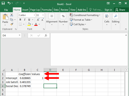
Now, we want to label the first empty column and add a “1” under the label. It should appear like the image below:
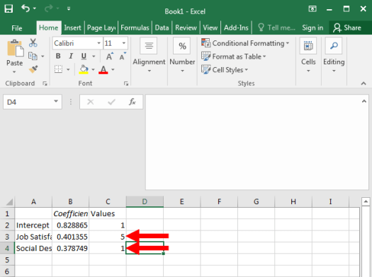
Then, you want to enter your specified values for job satisfaction and social desirability in the cells below the “1”. In this example, let’s choose the values of “5” for job satisfaction and “1” for social desirability. This means we want to predict the value of an employee’s job performance when their job satisfaction is 5 and their social desirability is 1.
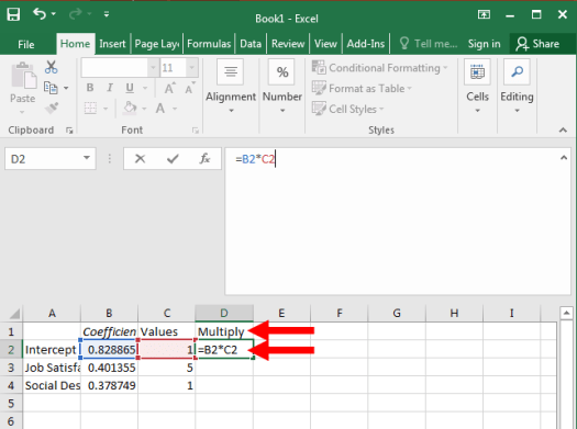
We now want to label the next column with the word “Multiply”, as we are going to use it to multiply the rows’ numbers together. Then, go ahead and multiply the two numbers in Row 2 together in this new column, as seen in the image below. It would probably be easiest to type “=B2*C2” to directly target the cells with the desired numbers.
Do the same for the next two rows.

Lastly, we want to label our final column as “Sum”, and we will want to use the =SUM() function to add the numbers together. To do so, type “=SUM(“, highlight the three numbers in the multiply column, type “)”, and then hit enter. Your result should look like the image below.

Did you get this number? If so, great! If not, try the guide again until you get the correct value.
From this result, we would expect a job performance value of 3.214 given a job satisfaction value of 5 and a social desirability value of 1. Thus, we were able to predict job performance given these values of job satisfaction and social desirability. Great work!
In other words, our equation steps looked like the following:
- y = .829 + .401(JS) + .379(SD)
- y = .829 + .401(5) + .379(1)
- y = .829 + 2.007 + .379
- y = 3.214
You can perform similar analyses using any type of regression output. If you ever need any help with this, please email me at MHoward@SouthAlabama.edu.
