Regression is a powerful tool.  Fortunately, regressions can be calculated easily in Excel.  This page is a brief lesson on how to calculate a regression in Excel.  As always, if you have any questions, please email me at MHoward@SouthAlabama.edu!

---

The typical type of regression is a linear regression, which identifies a linear relationship between predictor(s) and an outcome.  In other words, a regression can tell you the relatedness of one or many predictors with a single outcome.  Regression also tests each of these relationships while controlling for the other predictors, and it can be used to answer the following questions and similar others:

• What is the relationship of job satisfaction and leader ability in predicting employee job satisfaction?
• What is the relationship of hours studied and test grades?
• What is the relationship between NBA player height, weight, wingspan and the number of points scored per game?

Of course, there is more nuance to regression, but we will keep it simple.  To answer these questions, we can use Excel to calculate a regression equation.  If you don’t have a dataset, you can download the example dataset here. In the dataset, we are investigating the relationships of job satisfaction and social desirability with job performance.

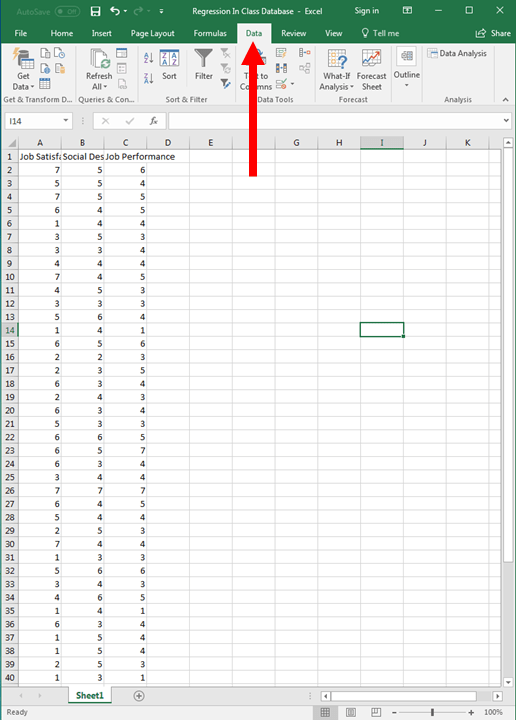
The data should look something like this:

If your dataset looks differently, you should try to reformat it to resemble the picture above. The instructions below may be a little confusing if your data looks a little different.

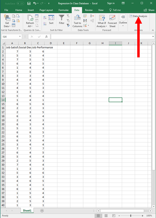
Once you have the data open, the first step is to click on the Data tab at the top. Then click on Data Analysis, as seen below:

Don’t see that tab? If not, go to my page on Activating the Data Analysis Tab. It should appear once you activate it.

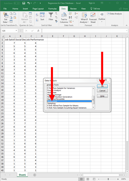
If it worked, the following window should have appeared.  You’ll want to click on Regression, and then press OK.

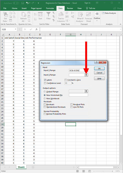
The following window should pop up.  On this window, you need to first click on the icon to identify your Input Y Range.  This represents your outcome data.  Then, you need to highlight (click and drag) your outcome data and labels.  Then press the icon again.  This will identify your relevant outcome data.

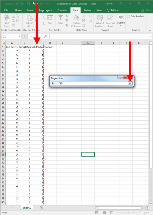
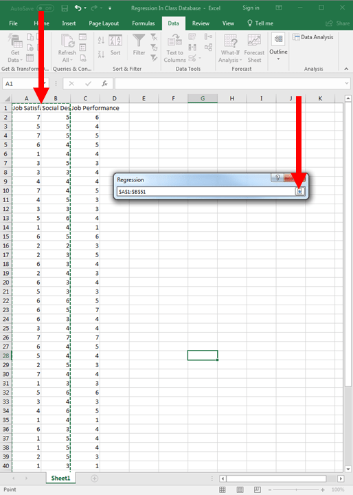
Next, you need to click on the icon to identify your Input X Range.  This represents your predictor data.  Then, you need to highlight (click and drag) your predictor data and labels.  Then press the icon again.  This will identify your relevant predictor data.

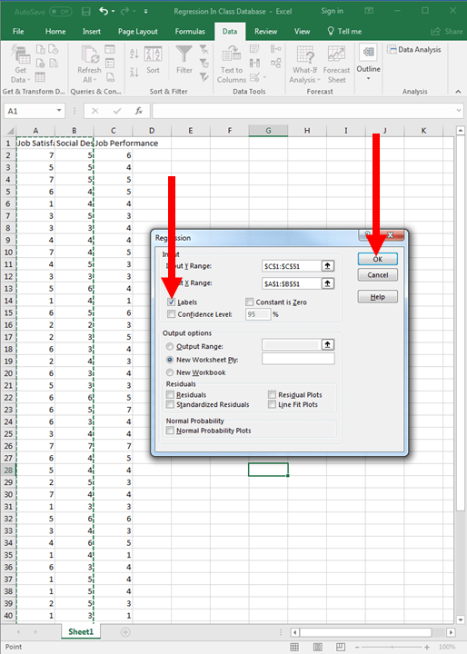
Now, click on Labels and then click on OK.

Now we get results!  They should look like the following.

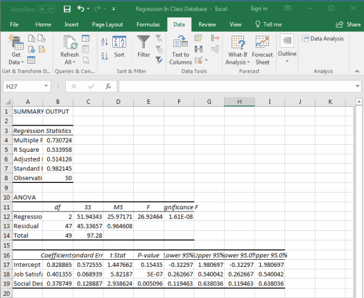
When reading the table below, we can look at the coefficients column to find the associated beta values.  From this table, we can see that the unstandardized beta for the intercept is .829.

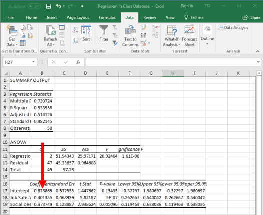
The unstandardized beta for job satisfaction is .401

And the unstandardized beta for social desirability is .379.

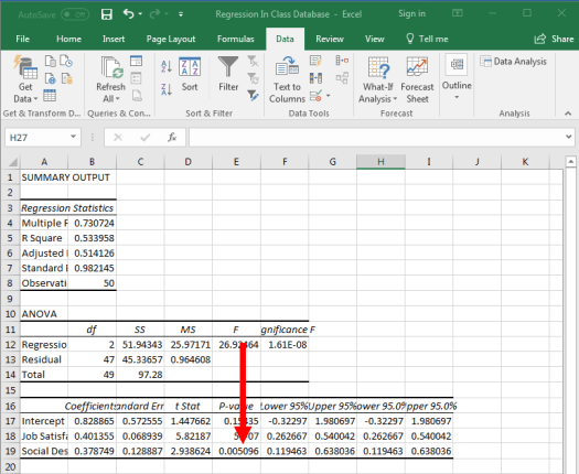
Also, we can use this table to determine the significance of our predictors.  The associated p-value of job satisfaction is less than .001.

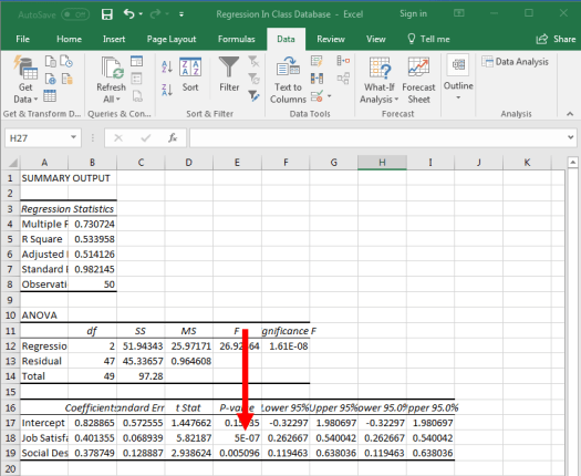
Also, the associated p-value of social desirability is less than .01.

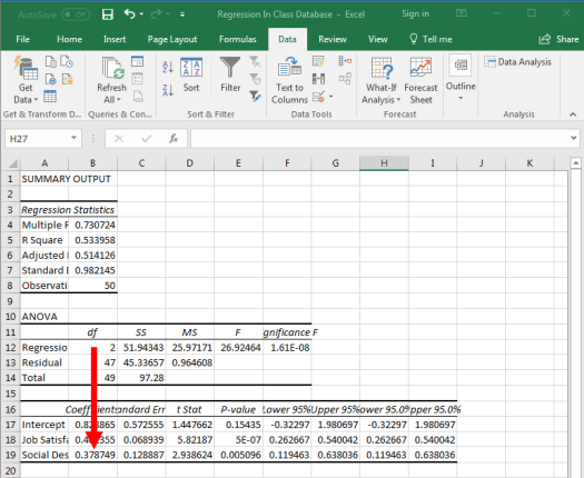
Lastly, we can see that the R-Square of the model is .53.

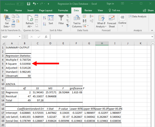
Together, the regression equation for these results is: y = .829 + .401(JS) + .379(SD); both job satisfaction and social desirability were statistically significant (p < .001 & < .01, respectively); and the total R-Square was .53 for the model.  Of course, the results provide other information, which may be useful for your certain purposes, but the current guide just covers the basics.

Now you should be able to perform a regression in Excel.  As always, if you have any questions or comments, please email me a MHoward@SouthAlabama.edu!