The chi-square test of independence, also called the two-variable chi-square test, is perhaps even more popular than the one-variable chi-square test.  Like the one-variable chi-square test, it is also one of the very few basic statistics that the “Data Analysis” add-on in Excel does not perform, and it is difficult to calculate without SPSS, R, or a different statistics program.  I created this guide on calculating the chi-square test of independence in Excel to help address this issue.  I hope that someone finds it helpful!  As always, email me at MHoward@SouthAlabama.edu if you have any questions about the chi-square test of independence.

---

As you likely already know, a one-variable chi-square test determines whether there is an equal (or unequal) number of observations across the categories of a single grouping variable.  If you don’t already know about one-variable chi square tests or how to perform them in Excel, then you should check out my guide on the topic (click here).

The purpose of a chi-square test of independence is a little bit different.  It determines whether the distribution of observations across the groups of one categorical variable (aka grouping variable) depends on another categorical variable.  Let’s look at a few examples to clarify this idea.

Imagine you have three people making toys (Sue, Joe, and Bob), and you record the number of defects in the manufactured toys (defect and no-defect).  In this example, you have two grouping variables: person and defect.  The person group has three categories (Sue, Joe, and Bob), and the defect group has two categories (defect and no-defect).  We could perform a chi-square test of independence to determine whether the defects are evenly distributed across all three people, or whether there is an unequal distribution of defects and one person my be producing significantly more or less than the others.  In this case, we would be testing whether the distribution of observations for our defect variable is dependent on our person variable.

Here is another example:  Imagine that you have four professors (Dr. Howard, Dr. Smith, Dr. Kim, and Dr. Chow), and you record the number of students that fail in these classes.  Again, we have two grouping variables: professor and pass/fail status.  The professor group has four categories (Dr. Howard, Dr. Smith, Dr. Kim, and Dr. Chow), and the pass/fail status group has two categories (pass and fail).  We could perform a chi-square test of independence to determine whether the failing students are evenly distributed across all four professors, or whether there is an unequal distribution of failing students and some professors may be producing significantly more or less than the others.  In this case, we would be testing whether the distribution of observations for our pass/fail variable is dependent on our person variable.

Two last notes about the chi-square test of independence before learning how to calculate it in Excel:  First, when I was taught it, I was taught that it tests whether there is an interaction between two categorical variables regarding the distribution of their observations.  If it helps you to think of it in this manner, then do so.  Second, the chi-square test seems similar to a t-test.  An easy way to remember the difference is that the chi-square test uses a categorical variable as your outcome, whereas a t-test uses a continuous variable as your outcome.  You could also say that the chi-square test uses the number of observations as your outcome, whereas a t-test uses a continuous variable as your outcome.

Now that we know what a chi-square test of independence is used for, we can now calculate it in Excel.  To begin, open your dataset in Excel.  Click here for the dataset that I will be using in the current example. It includes the gender and hair colors of 60 randomly sampled students, and we will be testing whether there is an association between gender and hair color regarding the number of observations for their respective categories. In other words, does the number of males or females depend on hair color and/or does the number of blonde- or brown-hair students depend on gender?

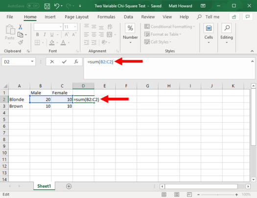
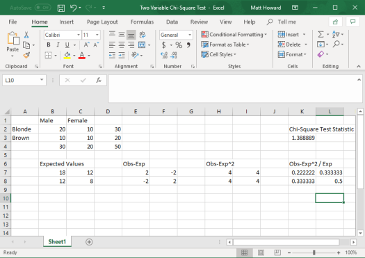
The data should look like the following:

First, you want to sum your rows and columns using the =SUM() command.  Let’s start with the top row.  To sum this row, select the cell next to the end of the row, as seen below.  Then type “=Sum(“, select the two cells that you want to sum, and then type “)”.  Do not include the quotation marks for any of these instructions. This will sum the row for you, as seen below:

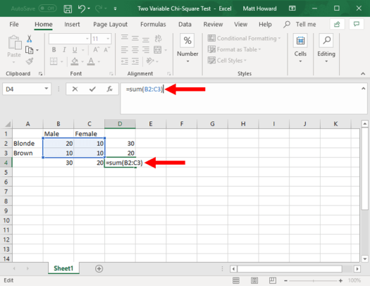
Now, we want to repeat this process for the other row and the two columns.  Just use the =SUM() command again using the same cells as below.

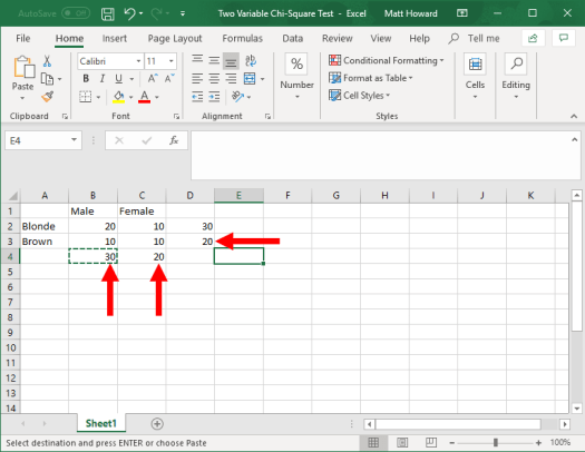
We then want to get the overall total of all observations.  Select the empty, bottom-right cell.  Then, use the =SUM() command, and select all four of the original cells.  This will give you the overall total of all observations, as seen below.

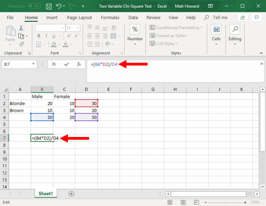
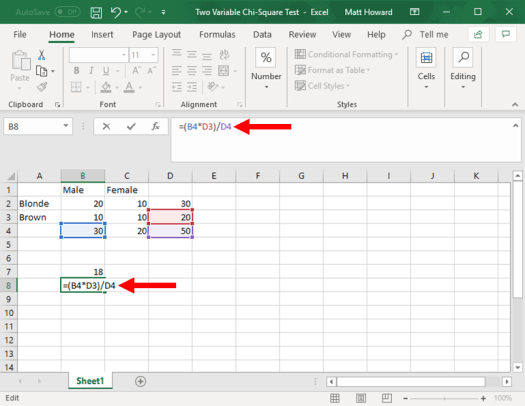
Now, we need to calculate the expected values for each cell.  To do so, we multiply the sum of the cell’s row times the sum of the cell’s column, then we divide by the total number of observations.  To do so for the upper-left cell, we first select a empty cell, such as the one highlighted below.  Then, we type “=(“, select the sum of the upper row, type “*”, select the sum of the left column, type “)/”, select the overall total of observations, and hit enter.  This will give us: =(B4*D2)/D4, as seen in the image below.

Now, we want to do the same for the other cells.  I will walk you through each one, as this part is a little complected.

To get the expected value for the bottom-left cell, we multiply the sum of the bottom row times the sum of the left column and divide by the overall total of observations.  You can see this in the image below, including the formula that you will use.

The image below includes the formula for the top-right cell.

And the image below includes the formula for the bottom-right cell.

Now let’s label these four new cells.  I used the label, “Expected Values”.

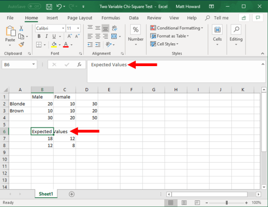
You should now have all four expected values and a label.  Good work!

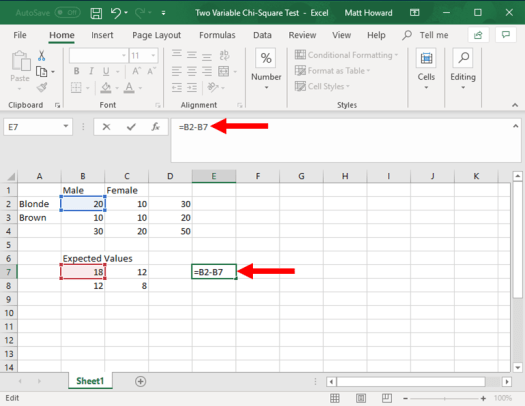
Now we want to subtract the original observed values by the expected values.  Let’s start with the upper-left cell again.  First select a blank cell, such as the one highlighted below.  Type “=”, select the upper-left observed value, type “-“, select the upper-left expected value, and hit enter.

Now, let’s repeat the process for the other three cells and give your new section a label.  I used the label, “Obs-Exp”.

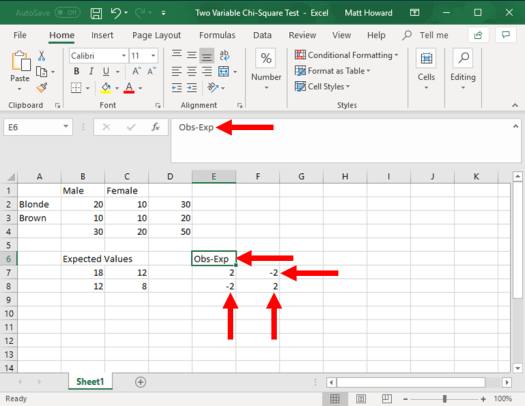
Does your observed minus expected values look like the image above?  If so, good work!  If not, go back and try it again.

Now, we need to square these new values, starting with the upper-left cell.  Again, select a blank cell.  Then type “=”, select the upper-left cell of the observed minus expected values, type “^2”, and hit enter.  To type “^”, just hold down shift and press the number 6 on your keyboard.

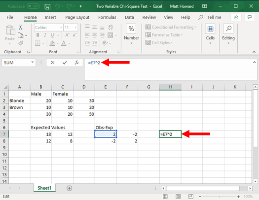
Now, let’s repeat the process for the other three cells and add a label.  I used the label “Obs-Exp^2”.

We now need to divide our newly created values by our expected values, starting with the upper-left cell.  Just click on a blank cell, type “=”. select the upper-left cell of your most recently created values, type “/”, select the upper-left cell of your expected values, and then hit enter.

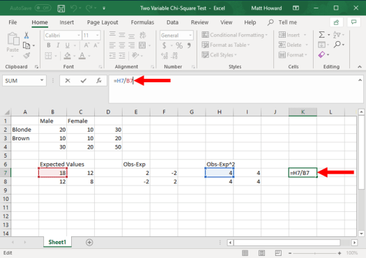
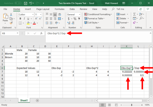
Again, repeat the process and add a label.  I used the label “Obs-Exp^2 / Exp”.

Lastly, we want to sum these most recent values.  Select a blank cell, type “=SUM(“, select your four newly created values, type “)”, and hit enter.

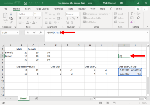
Finally, add a label.  I labeled this final value, “Chi-Square Test Statistic”.

Done with the calculations!  Take a look at the picture below.  Do your results look like this?  Did you get a final value of 1.388889?  Wonderful if you did!  Again, if you did not, take a look at the images above and see where your numbers differed.

So, what does a chi-square test statistic of 1.38889 mean?  Well, we need to use a chi-square significance table to find out!  To use this table (below), we need to determine our degrees of freedom as well as what we want our significance level (aka alpha) to be.

For a chi-square test of independence (two variables), our number of degrees of freedom is the number of rows minus one multiplied by the number of columns minus one.  This is expressed in the formula below:

• df = (#r – 1)*(#c – 1)

In this example, we would plug in the number two for both the number of columns and the number of rows.  This would give us the following:

• df = (2 – 1)*(2 – 1)
• df = (1)*(1)
• df = 1

So our degrees of freedom are 1.  What about our alpha?  We set this ourselves, and we almost always use a value of .05.  This is because we would only consider a result to be statistically significant if the p-value was less than .05.

When these numbers decided, we use the table below to find our chi-square test cutoff value. If our result is higher than the number on the table, then our results are statistically significant. So, in the picture below, find where the one degrees of freedom row intersects with the .05 significance level column.

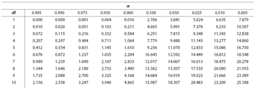
Did you find it?  The number is 3.841.  So, our result must be greater than 3.841 to be statistically significant.  Because our result was 1.388889, we can certainly say that it was not statistically significant.  This means that the two variables can be considered independent in regards to the distribution of their observations.  The number of observations for  gender did not depend on hair color, and the number of observations for hair color did not depend on gender.  The two variables are considered independent.

That is all for one-variable chi-square tests.  Hopefully this page was a little bit helpful!  If you still have questions, please contact me at MHoward@SouthAlabama.edu.