Many situations call for the one-variable chi-square test.  Unfortunately, it is one of the very few basic statistics that the “Data Analysis” add-on in Excel does not perform, and it is often a pain to calculate without SPSS, R, or a different stats program.  To help with this issue, I decided to create a guide on calculating a one-variable chi-square test in Excel.  It isn’t as easy as most other analyses in Excel, but I hope that you find it helpful.  Feel free to email me at MHoward@SouthAlabama.edu if you have any questions about performing a one-variable chi-square text in Excel.

---

So what does a one-variable chi-square test do?  It determine whether there is an equal (or unequal) number of observations across the categories of a single grouping variable.  Sound confusing?  Let’s look at a few examples.

Imagine that you have a classroom, and you count how many students are men and women.  In this example, you would have one grouping variable, gender, which has two categories, male and female.  You could perform a chi-square test to determine whether there is a statically significant difference in the number of men and women in the class.

Here is another example:  Imagine that you have 100 employees, and you ask them whether they are blue-collar, white-collar, or service employees.  In this example, you would have one grouping variable, occupation type, which has three categories, blue-collar, white-collar, and service.  You could perform a chi-square test to determine whether there is a statically significant difference in the number of blue-collar, white-collar, and service employees in the sample.

Now that we know what a chi-square test is used for, we can now calculate a chi-square test in Excel.  To begin, open your dataset in Excel.  Click here for the dataset that I will be using in the current example. It includes the hair colors of 100 randomly sampled students, and we will be testing whether there is a significant difference in the distribution of hair colors within the sample – blonde, brown, and red.

The data should look something like this:

The very first thing that we want to do is calculate the expected value for each cell.  To do this, we sum all the cells and divide by the number of cells – also known as taking the average of the cells.  In Excel, you can do this by using the =AVERAGE() command.  First, type “=AVERAGE(” (without quotation marks), then highlight the cells that you want to average, and then close your parenthesis by typing “)”.  Go ahead and do this for the first row.  You can see this in the picture below:

Now, do the same for the following two cells, and add a title for this column.  I used the title “Expected”, as this column represents the expected value for the cells.

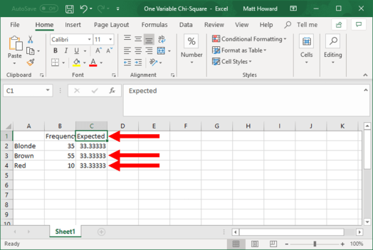
Did you get 33.33333 for each of the cells?  Great!  When performing a one-variable chi-square test, the expected value will always be the same for each of the cells.

Now, you want to add a new column, where you subtract the expected values from the observed values for each row.  To do this for the first row, you will want to type “=”, click on the frequency for the first row (35 in this example), type “-“, click on the expected value for the first row (33.33333 for this example), and finally hit enter.  This should give you “=B2-C2” in the cell, which will result in a value of 1.666667.

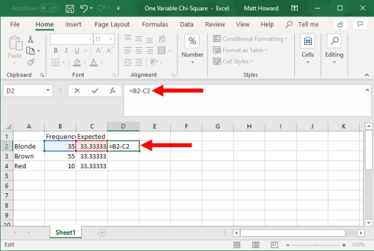
Now do the same for the other two rows and add a title to this column.  I use the title “Obs-Exp”, as this column represents the observed minus the expected values.

We want to square these values in the next column.  To do so, we type “=”, click on the on the cell that we want to square, type “^2”, and hit enter.  To type “^”, you simply hold down shift and hit the number 6.  We can see this done for the first row in the picture below.

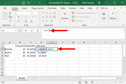
Let’s go ahead and do the same thing for the other rows and add a title.  I used the title “Obs-Exp^2”, because this row is the observed values, minus the expected values, squared.

Next, we need to divide these values by the expected values.  Let’s do this first the first row.  In the next column, type “=”, click on the “Obs-Exp^2” cell for the first row, type “/”. click on the “Expected” cell for the first row, and then hit enter.  You can see this in the picture below:

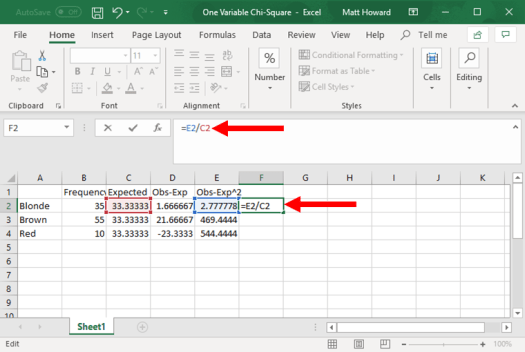
Go ahead and do the same for the other two cells in this column and add a title.  I used the title, “Obs-Exp^2 / Exp”, because that is exactly what this column represents.

For the last calculation, we need to sum the values in the last column using the =SUM() command.  To do so, type “=SUM(“, highlight the three cells in the final column, type “)”, and finally hit enter.

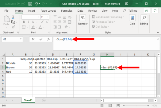
Lastly, add a title so we don’t forget what this number represents.  I used the title “Chi-Square Statistic”.

Phew!  We are all done with the calculations!  Did you get the number 30.5 as your result?  If so, great!  If not…go back and try it again.

So, what does this number mean?  Honestly, not a lot by itself.  To determine whether our result is statically significant, we need to compare our number to a chi-square significance table.  To use this table (below), we need to determine our degrees of freedom as well as what we want our significance level (aka alpha) to be.

For a one-variable chi-square test, the degrees of freedom is the number of groups subtracted by one.  We had three groups in this example, so our degrees of freedom would be two.  Alternatively, we set our significance level to be .05, as we would only consider a result to be statistically significant if the p-value was less than .05.

When these numbers decided, we use the table below to find our chi-square test cutoff value.  If our result is higher than the number on the table, then our results are statistically significant.  So, in the picture below, find where the two degrees of freedom row intersects with the .05 significance level column.

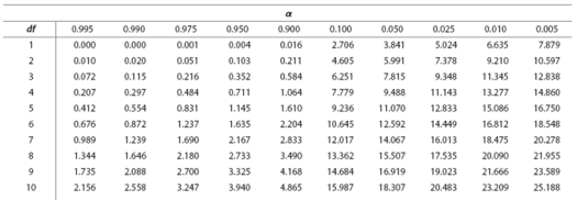
Could you find it?  It is the number 5.991.  So, our result must be greater than 5.991 to be statistically significant.  Because our result was 30.5, we can certainly say that it is statistically significant.  This means that we did not have an equal distribution of observations across the three groups.  In other words, we had an unequal distribution of observations across the three groups.

That is all for one-variable chi-square tests.  Hopefully this page was a little bit helpful!  If you still have questions, please contact me at MHoward@SouthAlabama.edu.