I often use two-sample t-tests as an introduction to SPSS in my undergraduate statistics courses – and sometimes my graduate courses, too.  Because the students are still getting used to functions in SPSS, they tend to have many difficulties with this lesson.  For this reason, I created the page below to provide an easy-to-read guide on performing two-sample t-tests in SPSS.  As always, if you have any questions, please email me a MHoward@SouthAlabama.edu!

---

Before learning about two-sample t-tests in SPSS, we must first know what a two-sample t-test is used for.  The textbook definition says that a two-sample t-test is used to “determine whether two sets of data are significantly different from each other”; however, I am not a fan of this definition.  Instead, I prefer to say that a two-sample t-test is used to “test whether the means of a measured variable in two groups is significantly different.”  So, a two-sample t-test is used to answer questions that are similar to the following:

• In our sample, do women have better test grades than men?
• Are men taller than women?
• Do people in a class taught by Dr. Howard perform better on a test than those in Dr. Smith’s class?
• Do employees in Training Group A have better performance than Training Group B?

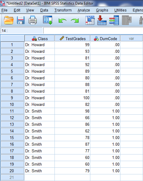
Now that we know what a two-sample t-test is used for, we can now calculate a two-sample t-test in SPSS!  To begin, open your data in SPSS.  If you don’t have a dataset, download the example dataset here. In the example dataset, we are comparing the test grades of two classes (Dr. Howard and Dr. Smith) to determine which class has higher grades on an exam.

The data should look something like this:

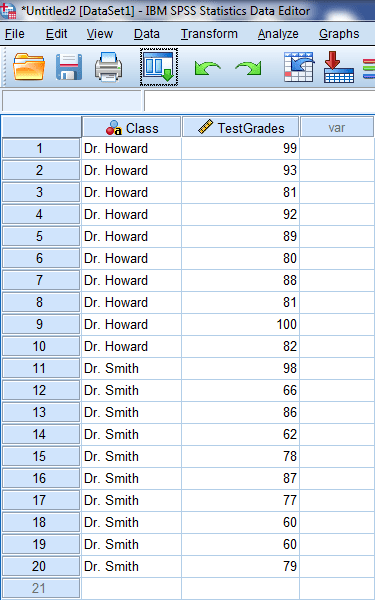
If it doesn’t, you may need to reformat your dataset.  It may be difficult to follow along if your dataset looks differently.

We first need to make a new grouping variable, because our current grouping variable in our dataset (Class) consists of fairly long text.  In SPSS, a two-sample t-test must be performed with a grouping variable that contains numerical values or very short text.  So, we need to create a new variable with 0s for everyone in Dr. Howard’s class and 1s for everyone in Dr. Smith’s class, which is called a dummy-coded variable.  Fortunately, creating a dummy variable is fairly easy.

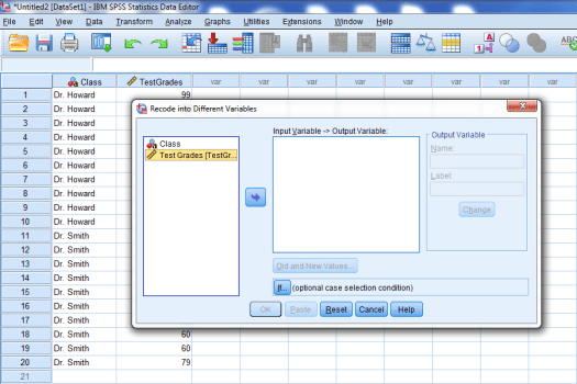
To start this process, click on Transform and then Recode into Difference Variables.

You should then have a window that looks like the one below:

We are going to recode the Class variable.  Click on Class, then click on the highlighted arrow.

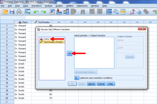
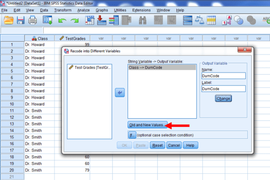
This will place Class in the other window, as seen below:

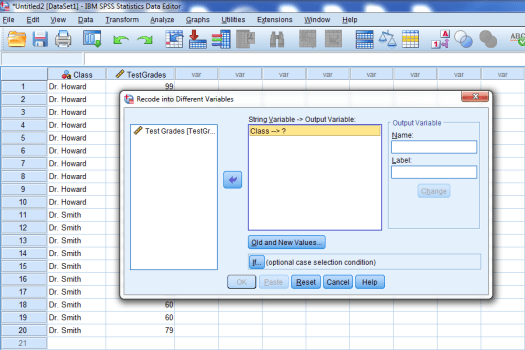
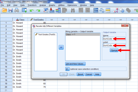
We then want to give our new dummy-coded variable a name.  Let’s call it DumCode.  To do so, type DumCode into the Name and Label boxes.  Then click Change.

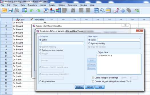
Afterwards, we want to assign the new values to our DumCode variable.  Click on Old and New Values.

The window seen below should pop up:

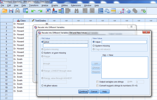
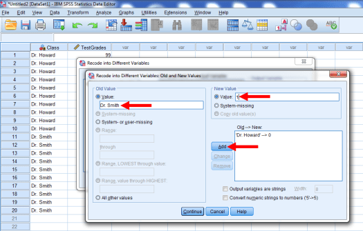
We want to recode our groups as 0 and 1.  To start, we’ll type Dr. Howard in the Old Value box, and we’ll type 0 in the New Value box.  Then, we’ll press add.

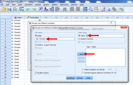
The result should look like the window below:

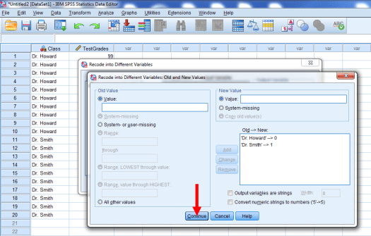
Now, we’ll type Dr. Smith in the Old Value box, and 1 in the New Value box.  Press Add again.

Press Continue.

And then OK.

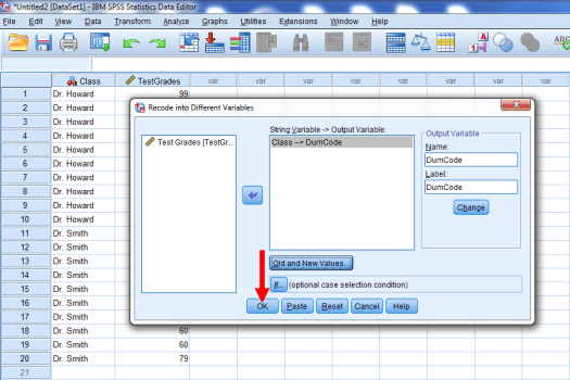
Does your data now look like the image below?  If so, great!  If not, review the instructions above to see what happened.  You’ll need this dummy-coded variable to perform the actual two-sample t-test.

To conduct the actual two-sample t-test, we’ll want to click on Analyze, Compare Means, and then Independent-Samples T-Test.

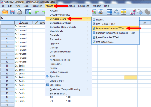
The following window should pop up.

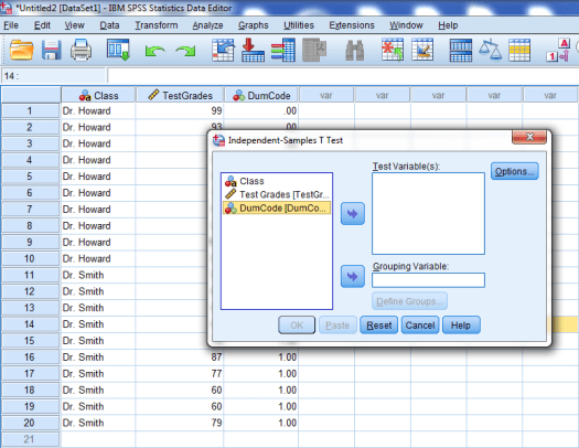
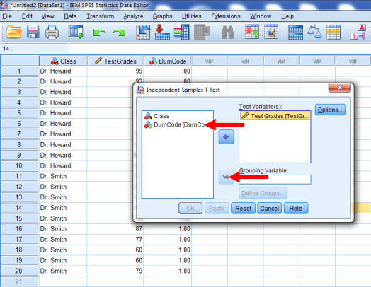
We’ll first want to put our outcome variable, Test Grades, into the test variable window.  To do so, click on Test Grades and then click on the arrow highlighted below.

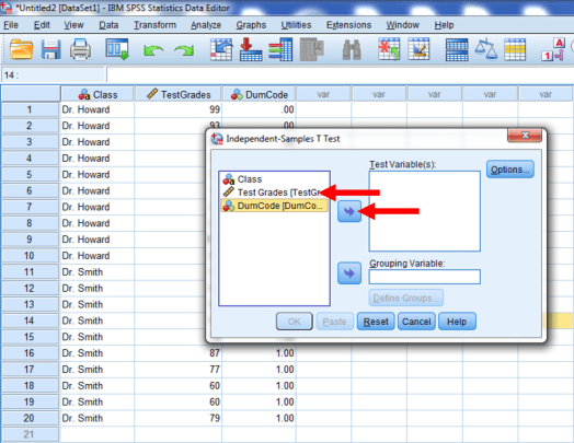
Next, we’ll want to identify our grouping variable.  Click on our dummy-coded variable, DumCode, and then click on the arrow highlighted below.

Once DumCode is in the Grouping Variable window, you’ll want to click on Define Groups.

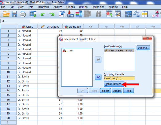
The following window should pop up.

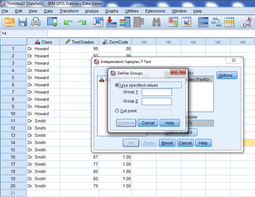
You’ll  want to enter the dummy-coded values, 0 and 1, into the Group 1 and Group 2 boxes, as seen below.  Then press continue.

Now press OK.

We should get results.  Yay!

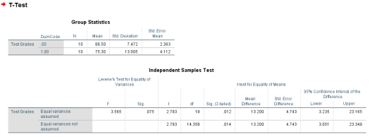
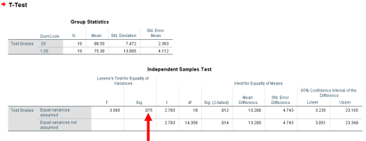
We’ll first want to look at Levene’s Test for Equality of Variances.  If it is significant, we cannot assume equal variances.  If it is not significant, we can assume equal variances.  From looking below, the p-value for Levene’s Test of Equality of Variances is not significant (p > .05), so equal variances can be assumed.

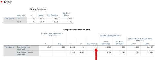
Looking at the equal variances assumed line, we can see that the results of the t-test are statistically significant (p < .05).  This indicates that a significant mean difference exists in the test scores of Dr. Howard’s class and Dr. Smith’s class; however, this result will not tell you which group scored higher.

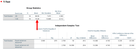
To determine the nature of this mean difference, we must look at the group means.  As we can see below, Group 0 had a much higher test average than Group 1.  If we remember our dummy-coded values, Dr. Howard was Group 0 and Dr. Smith was Group 1.  Thus, we can say that there is a significant difference in the mean test scores of Dr. Howard and Dr. Smith, with Dr. Howard’s class having higher grades than Dr. Smith.

Together, we can identify that…

• The test statistic is: 2.783
• The p-value is .012 (< .05)
• The mean of Dr. Howard’s class is 88.5
• The mean of Dr. Smith’s class is 75.3
• Dr. Howard’s class performed significantly better than Dr. Smith’s class.

We did it! We calculated everything that we needed to know about the two-sample t-test! Good work!

Do you still have any questions?  Or comments about this guide?  Feel free to email me at MHoward@SouthAlabama.edu.  I am always happy to chat!