Regression is a powerful tool.  Fortunately, regressions can be calculated easily in R.  This page is a brief lesson on how to calculate a regression in R.  As always, if you have any questions, please email me at MHoward@SouthAlabama.edu!

The typical type of regression is a linear regression, which identifies a linear relationship between predictor(s) and an outcome.  In other words, a regression can tell you the relatedness of one or many predictors with a single outcome.  Regression also tests each of these relationships while controlling for the other predictors, and it can be used to answer the following questions and similar others:

• What is the relationship of job satisfaction and leader ability in predicting employee job satisfaction?
• What is the relationship of hours studied and test grades?
• What is the relationship between NBA player height, weight, wingspan and the number of points scored per game?

Of course, there is more nuance to regression, but we will keep it simple.  To answer these questions, we can use R to calculate a regression equation.  If you don’t have a dataset, you can download the example dataset here.  This dataset does not include any missing data.  So, if you are dealing with missing data, you may have to add an extra command or two to your syntax.

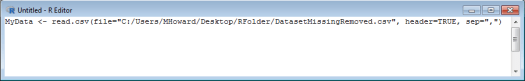
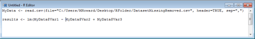
First, you need to open your data into R.  If you do not know how to do this, please refer to my page on opening .csv values into R.  Your syntax should now look something like this:

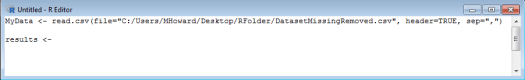
We can now type our command syntax.  To start, we are actually going to assign our results to a label, which will be useful later.  For this example, we are going to label our results as: results .  So, you should type: results <- .

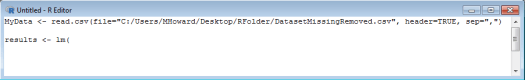
We want to type in our command, which is: lm( .

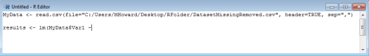
Now, we can type our regression model.  For the current example, we want Var1 to be our outcome, which should come first in the model.  To designate Var1 as our outcome, we would type: MyData$Var1 ~ .  We can refer to Var1 by typing MyData$Var1 because our dataset has labels.

Our predictors should be entered next, as separated by plus signs (+).  In the current example, we are going to use Var2 and Var 3 as our predictors.  So, we should type: MyData$Var2 + MyData$Var3 .

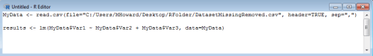
We should then enter a comma (,), and designate that we are using MyData as our dataset.  To do so, we would enter: , data=MyData .

Remember how we are assigning our results to the label “results”?  If we were to run the syntax above, it would just assign our results to the label “results” without actually telling us the results.  For this reason, we need to enter the following on a new line:  summary(results) .

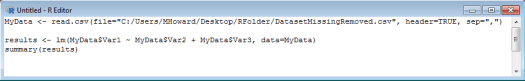
Run your syntax, and you should get something like the following:

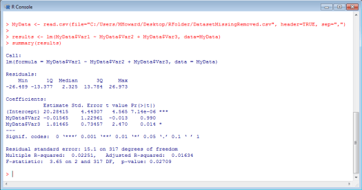
Did you?  If so, great!  Let’s look at these results.  First, in the coefficients section, we get an estimate for each predictor (beta), a standard error, a t-value, and a p-value.  From these results, we can see that Var2 was not a significant predictor of Var1, but Var3 was a significant predictor of Var1.  Interesting!  We can also see our overall model results, such as the multiple R^2, which may be of interest to some readers.

From this example, you should be able to run a regression on your own in R.  You can also use the example dataset to create different regression equations.  If you have any questions or comments while doing so, feel free to email me at MHoward@SouthAlabama.edu.