I don’t come across the need to perform a one-sample t-test that often, whether in research or practice.  However, it is a very good entry into learning about two-sample t-tests and ANOVAs, so I teach it early in my undergraduate statistics courses.  I get slightly annoyed whenever I teach it, though, because Excel does not have the one-sample t-test built into its Data Analysis add-on.  Nevertheless, we can trick Excel into performing it for us, which I detail below.  If you have any questions, please email me at MHoward@SouthAlabama.edu.

---

The purpose of a one-sample t-test is pretty simple.  It tells us whether the mean of a variable is significantly different than a chosen value, and it can be used to answer the following questions:

• Is a basketball team’s average height significantly different than 6’6″?
• Is a company’s yearly revenue significantly different than 10 million dollars?
• Is the job satisfaction of a company’s employees significantly different than a 4 on a 1 to 7 scale?

These questions may be interesting, but they don’t occur all that often in research or practice, and selecting an arbitrary value to test isn’t typically informative.  Nevertheless, some examples in which a one-sample t-test may be useful are:

• When you know a pre-defined value is important.
• When you have a certain expected value for a sample.
• When there is some common-sense value.
• When you are performing a replication study.

Of course, there are other situations in which a one-sample t-test may be useful, so keep your eyes open for these situations!

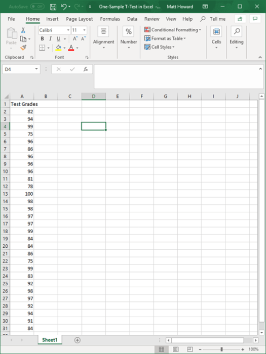
Now that we know what a one-sample t-test is used for, we can now calculate a one-sample t-test in Excel.  To begin, open your data in Excel.  If you don’t have a dataset, download the example dataset here. In the example dataset, we are comparing the test grades of a class to the chosen value of 80. This will determine whether the students’ average grades are significantly different from a value of 80.

The data should look like the image below.

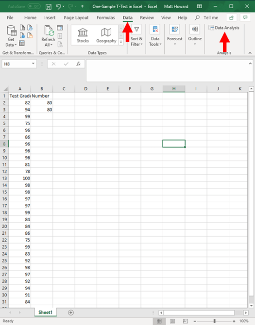
Now, we need to start by tricking Excel into calculating the one-sample t-test for us.  Let’s start by typing three things into the second column.  In the first row, type the word “Number” (without quotation marks), which is our label.  In the second and third row, type the number that you want to compare the data against.  In the current example, we chose the number “80”.  So, type “80” (without quotation marks) into the second and third rows of the second column.  Your Excel should look like the image below:

With the numbers entered, now click on the Data tab at the top, and then click on the Data Analysis button.  If you do not have this in your version of Excel, check out my page on Activating Data Analysis in Excel.

The following window should pop up.  This is where it gets a little confusing.  Although we are performing a one-sample t-test, you should click on “t-Test: Two-Sample Assuming Unequal Variances” and then click on “OK”.  Because Excel does not have a one-sample t-test command, we must trick it into thinking those two numbers that we typed are another sample.  Confusing, I know, but it works!

Now, click on the button highlighted below:

And then click and drag overtop all the data in Column A.  In this example, I do NOT include the label.  Just click and drag on the numbers in the first column, and then press the highlighted button.

Click on the other button highlighted below:

And do the same thing, but highlight the numbers in the second column.  If you are using the example dataset, you should highlight the two number 80s.  Then press the highlighted button.

Press OK.

You should get results.  Yay!  Take a look at the image below and compare your results.  Did you get the same numbers?  If so, great!  If not, start from the beginning and try it again.

So what do these numbers tell us?  First, look at the highlighted number below.  In the current example, we have an average of 90.9.  This means the class’s test grade was, on average, a 90.9.  Already, we can tell that this is larger than our chosen number of 80.

Now, look at the number highlighted in the picture below.  This is our t-statistic.  It is our primary result or effect size, and it is 7.630 in the current example.  Is that big?  Is it small?  It is fairly difficult to interpret, so it would be best to turn to our p-value.

The number highlighted below is our p-value.  It is listed as 2.01E-08.  How does a number have an “E” in it?  Well, when a number is extremely small or large in Excel, it is sometimes reported in scientific notation.  The number after the E represents how many spaces we should move the decimal point.  If it is positive, we move the decimal to the right and make the number bigger.  If it is negative, we move the decimal to the left and make the number smaller.

So, the current result of 2.01E-08 is actually .0000000201. That is very, very small for a p-value – much less than our cutoff of .05.  Because our p-value is less than .05, then we would consider our results statistically significant.  If a one-sample t-test result is statistically significant, we would say that our mean is significantly different than the chosen value.  In the current example, we would say that the class average is significantly different than a value of 80.  Then, we could look at the mean (90.9) to determine that our class mean is significantly larger than a value of 80, because the mean is both significantly different and larger than a value of 80.

That is all for the one-sample t-test in Excel!  If you have any questions, please contact me at MHoward@SouthAlabama.edu.