
T-tests are used to identify the mean difference between two groups. But what do you do if you want to compare the mean difference of more than two groups? Well, as you’ve probably guessed, you can perform an ANOVA. Because ANOVA is a commonly-used statistical tool, I created the page below to provide a step-by-step guide to calculating an ANOVA in Excel. This page is for a one-factor ANOVA, which is when you have a single grouping variable and a continuous outcome. As always, if you have any questions, please email me a MHoward@SouthAlabama.edu!
As mentioned, an ANOVA is used to identify the mean difference between more than two groups, and a one-factor ANOVA is used to identify the mean difference between more than two groups when you have a single grouping variable and a continuous outcome. So, a one-factor ANOVA is used to answer questions that are similar to the following:
- What is the mean difference of test grades between Dr. Howard’s class, Dr. Smith’s class, and Dr. Kim’s class?
- What is the mean difference in total output of five different factories?
- What is the mean difference in performance of four different training groups?
Now that we know what an ANOVA is used for, we can now calculate an ANOVA in Excel. To begin, open your data in Excel. If you don’t have a dataset, download the example dataset here. In the example dataset, we are simply comparing the means of three different groups on a single continuous outcome. You can imagine that the groups and the outcome are anything that you want.
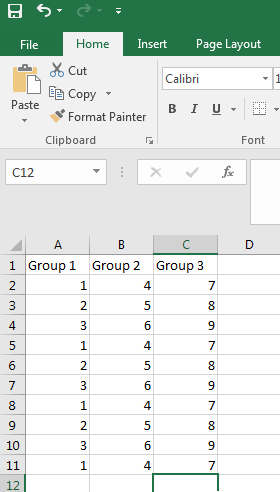
If you data doesn’t look like this, you should probably reformat it to appear similarly. Calculating an ANOVA in Excel may be a little difficult with different data formats.
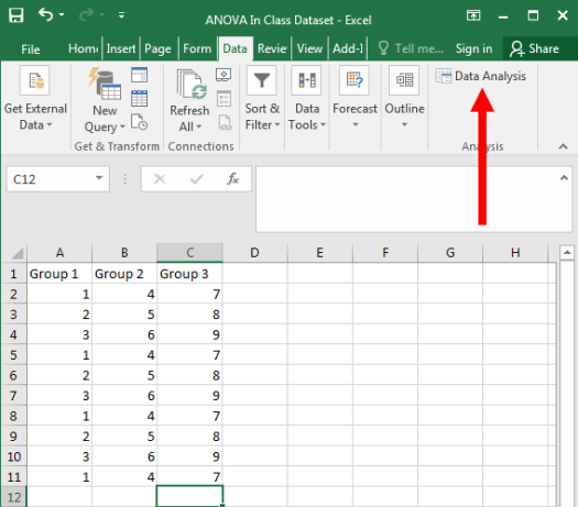
Like most analyses in Excel, we are going to start by clicking on the Data tab at the top, followed by clicking on the Data Analysis button.
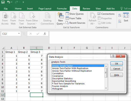
If it worked, the following window should have appeared. You’ll want to click on Anova: Single Factor, and then press OK – as seen below:
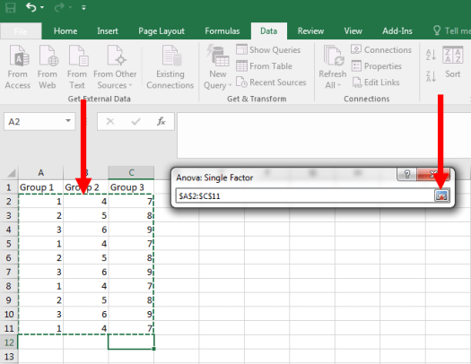
Then, the following window should pop up. On this window, you first need to click on the icon highlighted below to identify your data range. So, click on the button…
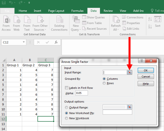
…and then highlight your data, and click the highlighted button. NOTE: You can highlight the labels too, if you want your results to be labeled. Make sure you click on the labels checkbox in the following window if you do so, however.
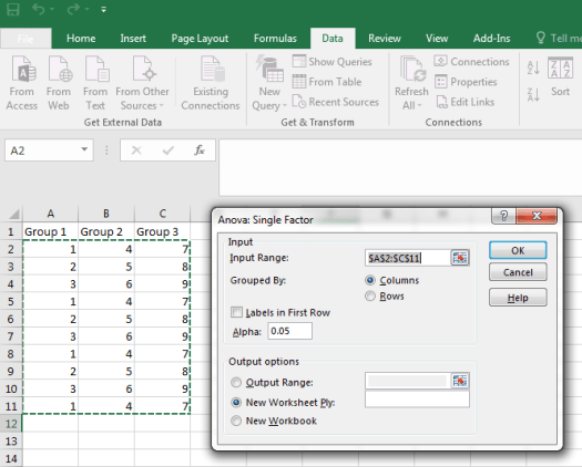
Now, with our data selected, we can press OK. NOTE: If you highlighted your labels when identifying your data, make sure you click on the checkbox for Labels in First Row. Then press OK.
As seen below, we should get results. Nice!
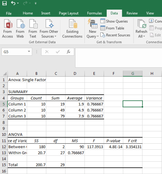
First, we should look at the effect size, which is the F-value. This is 117.391. When reporting our results, we would probably include this value, but it is difficult to interpret by itself…

…For this reason, we’ll also want to look at the p-value. In this example, it is extremely small (p < .0001), which indicates that our result is statistically significant. In the context of ANOVA, this means that there is a significant difference among the means of our groups. We would report this p-value as well as our interpretation of the result.

While we know that there is a significant difference among the groups, our F-value or p-value does not tell us the nature of these differences – only that some difference exists.
The best method to understand the nature of these differences would be to conduct post hoc tests. Unfortunately, Excel does not have an easy method to calculate post hoc tests. So, we’ll instead just look at the means relative to their variances, which can also be found in our results.

We can clearly see that the group differences are large relative to the variances of the groups. The groups’ variances each equal .767. The difference between Group 1 and 2 is three, the difference between Group 2 and Group 3 is three, and the difference between Group 1 and 3 is six. Given the small size of the groups’ variances, these differences very large. While this may not be clear at first look, the size of these group differences becomes more clear when you perform more ANOVAs.
That’s all for performing an ANOVA in Excel. As always, if you have any questions or comments, please email me at MHoward@SouthAlabama.edu.
