Whether for research or business, almost everyone runs descriptive statistics to begin their analyses.  I often see people use individual commands in Excel [i.e. =AVERAGE(), =STDEV()] to obtain these initial descriptives, but there is a much easier way to do this.  Thus, I wrote the guide below to running descriptive
statistics in Excel.  If you have any questions or comments, feel free to email me at MHoward@SouthAlabama.edu!

Descriptive Statistics are numerical indicators that detail certain aspects of your data.  These may include mean, median, mode, variance, standard deviation, and so forth.  We often want to run descriptive statistics to (a) obtain an initial
understanding of our data (b) and ensure that our data is correct.  For instance, imagine that we collected data and calculated the mean of a variable labeled “Age.”  The resultant value was 21.  We could then assume that our sample was fairly young – perhaps college students.  But what if the mean value was 1998?  Then we would assume that the variable was coded as “year of birth”  Even yet, what if the mean value was 10,000?  We could probably assume that something is wrong with our data.  So, just from the mean, we can know a lot about our data.

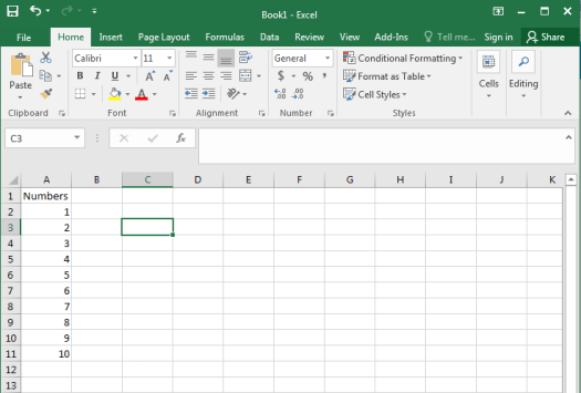
Now, let’s learn how to calculate descriptive statistics in Excel.  To begin, open your data in Excel.  If you don’t have a dataset, just copy or type the data below.  Don’t forget to include the label!

When you open your data in Excel, it should look something like this:

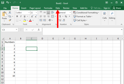
Once you have the data open, click on the Data tab at the top.  Look at the picture below if you need help finding it.

Then, click on the Data Analysis button, as seen below.

Don’t see this tab? If not, go to my page on Activating the Data Analysis Tab. It should appear once you activate it.

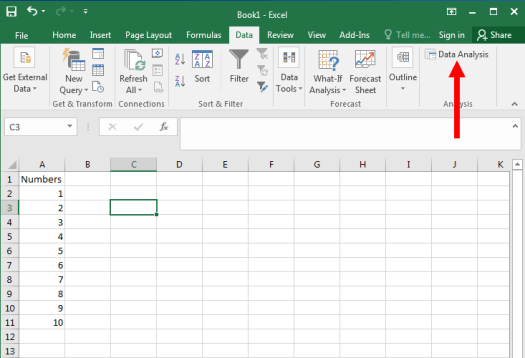
If you could see the tab, a new window should pop up.  Yay!  Now click on
“Descriptive Statistics” and press “OK.”

Once again, a new window should pop up.  Does it look like the one below?
In this window, click on the button highlighted below.

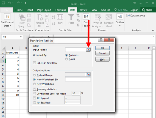
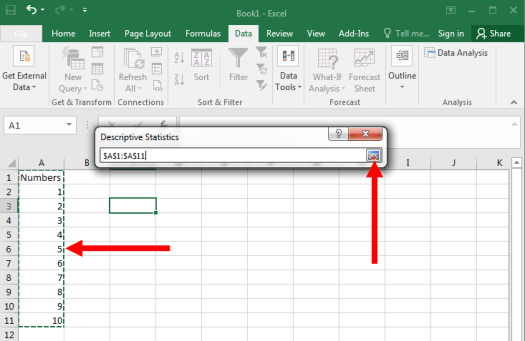
Now, highlight your data (including the label!), and press the other highlighted
button seen below.

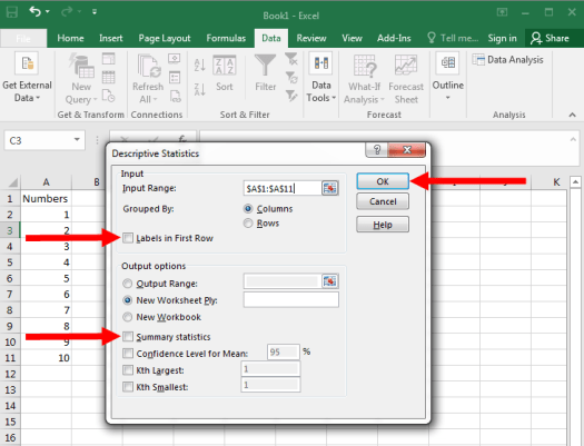
Before hitting the final “OK” button, you need to click two boxes.  Make sure you click the box “Labels in First Row” as well as the box “Summary Statistics.”  Once both of these boxes are checked, click the “OK” button.

Now, you should get output that looks like this:

Did you get something that looked like this?  If so, wonderful!  If not, try to go back from the beginning and start again.  If you still can’t get it to work, feel free to email me at MHoward@SouthAlabama.edu and I can try to help.

So, from our results, we can tell that our:

• Mean = 5.5
• Median = 5.5
• Mode = N/A
• Standard Deviation = 3.03
• Kurtosis = -1.2
• Skewness = 0
• Range = 0
• Count = 10
• And many more!

Hopefully this should provide all the descriptive statistics that you need.  If you need information or help with these, again, feel free to  contact me at MHoward@SouthAlabama.edu.  I’ll try my best to answer any questions!